Preparing data
In this notebook, we process interferometric measurement sets and create one-dimentional azimuthally averaged visibilities. If you already have such data, please proceed to the next section.
1. Import modules
We import frappe and some modules first.
[ ]:
from frap import msdata
import casatasks
import casatools
2. Process data
The CASA measurement sets have sometimes very complex structure. For a simple treatment, we first split the dataset into individual spectral windows.
[9]:
ms = msdata.ms( casatools = casatools, casatasks = casatasks )
[14]:
splitted_vis = ms.split( vis = './HD169142_band9.ms', datacolumn='DATA', dryrun = False )
Created working directory: ./working_HD169142_band9
splitted_vis stored the paths of the splitted ms. If dryrun == True , the function just returns the expected paths without actually splitting the ms.
[15]:
splitted_vis
[15]:
['./working_HD169142_band9/spw_id_0.ms',
 './working_HD169142_band9/spw_id_1.ms',
 './working_HD169142_band9/spw_id_2.ms',
 './working_HD169142_band9/spw_id_3.ms',
 './working_HD169142_band9/spw_id_4.ms',
... [Output Truncated]
We now want one-dimenional binned visibilities ( \(V(q)\) ).
get_visibilities() performs fitting of a two dimensional plane to visibility points inside a limited region on the frequency-uv space to estimate visibility values at representative coordinates, and saves them as a pickle file.
In this example, we have a band 9 data. Therefore,
[16]:
ms.get_visibilities( vis = [splitted_vis],
                     nu = [671.0e9],
                     pa = 6.31,
                     incl = 6.28,
                     FoV = 10.0,
                     output = 'HD169142_band9'
                   )
Processing fitting: 100%|████████████████████| 340/340 [00:02<00:00, 119.73it/s]
Saved visibility data to HD169142_band9.pkl
Sucesfully saved! In this case, we assumed that one frequency is enough to represent the whole data (i.e., the whole frequency range is small and linear approximation is valid). However, for instance, lower frequnency bands may have a much larger relative band width. In this case, you can make multiple channels by running:
[ ]:
# we do not run this cell in this notebook
ms.get_visibilities( vis = [splitted_vis1, splitted_vis2],
                     nu = [669.0e9, 672.0e9],
                     pa = 6.31,
                     incl = 6.28,
                     FoV = 10.0,
                     output = 'HD169142_band9'
                   )
Here, for example, splitted_vis1 and splitted_vis2 correspond to the lower and upper side bands, respectively, and the two frequencies are used to represent them.
Annyway, let’s check the results. You can access to the saved file with pickle.
[17]:
import pickle

with open('HD169142_band9.pkl', 'rb') as f:
    data = pickle.load(f)

q = data['q'] # uv-distance in lambda
V = data['V'] # visibility in Jy
s = data['s'] # uncertainty of V
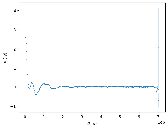
[18]:
import matplotlib.pyplot as plt

inu = 0
plt.errorbar(q[inu], V[inu], yerr = s[inu],
             capsize=0.1, fmt='o', markersize=1, elinewidth = 0.3 )


plt.xlabel(r'$q\ ({\rm \lambda})$')
plt.ylabel(r'$V\ ({\rm Jy})$')
[18]:
Text(0, 0.5, '$V\\ ({\\rm Jy})$')